Data pre-processing for machine learning models using scikit-learn & Python, Part 1

Hello readers! Lately, I have been completely immersed in Machine Learning and AI. Like a lot of us, I am captivated by what this thriving technology can do for us and how this allows me to expand my technical knowledge to places I never thought possible.

Usually, between 5am to 7am (when I am writing this post), you can find me in a coffee shop working on various technical projects that cover Machine Learning, AI, Database design, Mobile development and architecture, building my own IOS/Android budgeting app under the umbrella of my new business (more to come on this) and tons more. In those morning sessions, a few of them are dedicated to a Machine Learning class on Udemy I have been taking called Machine Learning A-Z: AI, Python & R + ChatGPT Bonus [2023]. If you are at all interested in Machine Learning, I think this course is a great starting point.

The post today is meant to cover some data preprocessing techniques that I have been using while building my own Machine Learning model with pytorch. My hope is that it could help inform someone else or equally better, help me grow by someone else’s feedback. Let’s not waste anymore time and jump right into the weeds!

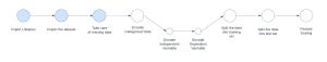
Process Diagram

Here is a simple diagram of the overall process. In this post for Part 1, we will only focus on the circles highlited with light blue:

Problem we are solving

Let’s say that I am a Machine Learning engineer at my company and marketing just pinged me on our company messaging service saying that they would like to launch a new campaign about buying cars, however they are not sure which target market they should appeal to. They have provided me with two data sets.

The first dataset contains data about people from different countries, their age, and their salary.

The second dataset includes all of the information from the first, but with one more column: Purchased

The marketing team would like me to build a model that shows the likelihood of people in the first data set that would purchase a vehicle based on data from the first dataset.

Lets get started!

Importing Libraries

There are so many libraries spinning up daily that help us preprocess our data prior to training models. For the examples in this post, I am going to use a variety of these libraries below. FYI – this get progressively more complex as they go along and I will explain beneath the imports what these are in general and what they will be used for in our application.

import numpy as np
import pandas as pd
from sklearn.compose import ColumnTransformer
from sklearn.preprocessing import OneHotEncoder
from sklearn.preprocessing import LabelEncoder
from sklearn.model_selection import train_test_split
from sklearn.preprocessing import StandardScaler
from sklearn.impute import SimpleImputer

• numpy: universal standard for working with numerical data in Python

  • Application usage: converting independent variables in our dataset to a numpy array for eventual compatibility with our model

• pandas: a fast, powerful, flexible and easy to use open source data analysis and manipulation tool

  • Application usage: reading our dataset into the python file for data preprocessing

• sklearn: an open source machine learning library that supports supervised and unsupervised learning. It also provides various tools for model fitting, data preprocessing, model selection, model evaluation, and many other utilities. Per the sklearn documentation, they have asked for a cite for usage of its API: API design for machine learning software: experiences from the scikit-learn project, Buitinck et al., 2013.

  • ColumnTransformer from sklearn.compose: Applies transformers to columns of an array or pandas DataFrame.

    • Application usage: ColumnTransformer allows us to pass our OneHoteEncoder class to transform/encode a set of dataset indices (usually categorical) into a one-hot numeric array.

  • SimpleImputer from sklearn.impute: Univariate imputer for completing missing values with simple strategies. Replace missing values using a descriptive statistic (e.g. mean, median, or most frequent) along each column, or using a constant value.

    • Application usage: We will use the SimpleImputer to find all missing values within our dataset and replace them with the mean of the values existing within the column.

  • LabelEncoder from sklearn.preprocessing: Encode target labels with value between 0 and n_classes-1. This transformer should be used to encode target values, i.e. y, and not the input X.

    • Application usage: We use this import to convert the dependent variable data column into a normalized data format for our eventual model use.

  • OneHotEncoder from sklearn.preprocessing: The input to this transformer should be an array-like of integers or strings, denoting the values taken on by categorical (discrete) features. The features are encoded using a one-hot (aka ‘one-of-K’ or ‘dummy’) encoding scheme. This creates a binary column for each category and returns a sparse matrix or dense array (depending on the sparse_output parameter)

    • Application usage: Take our categorical data and encode it into a binary column for each category. This encoding is needed for feeding categorical data to many scikit-learn estimators.

  • train_test_split from sklearn.model_selection: Split arrays or matrices into random train and test subsets.

    • Application usage: splitting our dataset into an 80/20 split for training and testing

  • StandardScaler from sklearn.preprocessing: Standardize features by removing the mean and scaling to unit variance.

    • The standard score of a sample x is calculated as: z = (x – u) / s

    • Application usage: using standardization in feature scaling to normalize our train and test data before we send it into our model

Importing the dataset

There are multiple ways to do this within a python file, however the method I chose for these exercises is using pandas. Please refer to the code below:

# Load the Iris dataset
df = pd.read_csv('iris.csv') # use read_csv panda function to load the data set into the python file

‘pd’ refers to the alias that i assigned to the pandas package after importing it. ‘df’ is just a plain variable assignment in Python. read_csv is a function provided by the pandas library to import your dataset. Notice that I do not have a path established in the argument that I am providing to the read_csv function and that is because it is locally stored in the same directory as my python file. If your dataset lived elsewhere, you would need to traverse to get it.

Here is a sample of the dataset for context (Its very simple for the sake of this write up):

CountryAgeSalaryPurchasedFrance4472000NoSpain2748000YesGermany3054000NoSpain3861000NoGermany40YesFrance3558000YesSpain52000NoFrance4879000YesGermany5083000NoFrance3767000YesSpain5776000No

Segmenting your data

In my specific datasets that I am working with, there are features and dependent variable vectors (last column). Features (independent variables) are the columns that we will use to predict the dependent variable (usually in the last column). In my examples, I will be using the iloc method that pandas provdes to extract the columns. Here is a nice explanation that I found on stack overflow that I really liked about the differences between using loc and iloc:

The main distinction between the two methods is:

• loc gets rows (and/or columns) with particular labels.

• iloc gets rows (and/or columns) at integer locations.

To demonstrate, consider a series s of characters with a non-monotonic integer index:

>>> s = pd.Series(list("abcdef"), index=[49, 48, 47, 0, 1, 2]) 
49    a
48    b
47    c
0     d
1     e
2     f

>>> s.loc[0]    # value at index label 0
'd'

>>> s.iloc[0]   # value at index location 0
'a'

>>> s.loc[0:1]  # rows at index labels between 0 and 1 (inclusive)
0    d
1    e

>>> s.iloc[0:1] # rows at index location between 0 and 1 (exclusive)
49    a

In our case, I used the iloc method to collect the matrix of features at the indexes of all the columns except dependent variable.

X = df.iloc[:, :-1].values # matrix of features -> iloc collects indexes of all the columns except dependent variable

Next, I used the iloc method to get the dependent variable vector from the imported dataset

y = df.iloc[:, -1].values # get the dependent variable vector

Its important to note that machine learning model that will eventually use these datasets will expect these 2 separate entities

Taking care of missing data

One obvious option to handle our missing data is to remove it from the dataset. One important consideration: This approach might not be too impactful if the percentage of missing data is tiny relative to your overall dataset and will not cause impact the learning quality of the model, but what happens if could be impactful?

Another option is to replace the missing data by the average of the data in your columns. This is the approach we will take here since removing any data from the dataset mentioned above could have serious implications on the learning quality of the model. Another important note: there are many other approaches to this (some that I have not even learned yet), however this is the approach we are taking for this specific dataset.

Here, we will use the SimpleImputer class to help us replace the missing data with the average of the column. By the way, one assumption that we are making here is that the missing data is indeed in the form of a nan and not something else that we would need to consider when remedying missing data.

One important item to mention that ChatGPT reminded me about when I put my post into a prompt for feedback was to talk about Hyperparameter tuning.

Hyperparameter tuning is the process of selecting the optimal hyperparameters for a machine learning model. Hyperparameters are parameters that are set before the learning process begins, and they determine how the learning algorithm behaves during training. Unlike model parameters, which are learned from the data (e.g., coefficients in linear regression), hyperparameters are not learned but need to be specified by the user.

Examples of hyperparameters in various machine learning models include:

1. Learning rate: A hyperparameter used in gradient-based optimization algorithms (e.g., stochastic gradient descent) that controls the step size at each iteration.

2. Number of hidden layers and neurons: In neural networks, the architecture of the network, such as the number of hidden layers and the number of neurons in each layer, are hyperparameters.

3. Regularization strength: Hyperparameters like L1 or L2 regularization strength in linear models or neural networks control the amount of regularization applied to the model.

4. Kernel type and parameters: In support vector machines (SVMs), the choice of kernel (linear, polynomial, radial basis function, etc.) and its associated parameters are hyperparameters.

5. Number of trees and depth: In decision tree-based models like random forests or gradient boosting machines, the number of trees and the maximum depth of each tree are hyperparameters.

6. Batch size: In deep learning, the batch size used during training is a hyperparameter that determines the number of samples processed before updating the model’s parameters.

The imputer discussed here does not have any hyperparameter tuning, however its still worth mentioning.

from sklearn.impute import SimpleImputer # this library will help us replace the missing data with the average of the column

imputer = SimpleImputer(missing_values=np.nan, strategy='mean')

imputer.fit(X[:, 1:3])

X[:, 1:3] = imputer.transform(X[:, 1:3]) #will be replaced by the meaan of the values in the column with missing data

In the code above, we are using the SimpleImputer class and searching for all values that have a missing value of nan. This might require some pre-work to your dataset to get it prepared for imputing. Another option that the SimpleImputer supports is a missing value of NA.

Where do we go from here?

This is where I am going to leave you for now. Mostly because I am a dad now and the amount of time that I get to sit down and write a lengthy blog post is shorter than it used to be. Here is what we will cover in Part 2:

• Encoding Categorical Data

  • Encoding the independent variable

  • Encoding the dependent variable

• Splitting the data into the training and test set

• Feature Scaling

Whats beyond Part 1 and Part 2?

Beyond Part 1 and 2, I. am going to be focusing on writing blogs that cover the following models:

• Linear Regression

• Multiple Linear Regression

• Polynomial Regression

• Support Vector Regression

Be on the lookout for blogs that cover this too!

Sneak peak to the code that supports these concepts

Check out the Data-Preprocessing-py-ml public github repo. I will be updating it more this week in anticipation for the Part 2 of this blog.

If you have made it this far, I really appreciate it and if there is any feedback you have, do not hesitate to reach out and strike up a conversation.

What does ChatGPT think of this blog?

ChatGPT seems to be fairly happy with my content and this is what it recommended for me to add or revise:

1. Explanation of Techniques: The article could benefit from providing more detailed explanations of the various data preprocessing techniques. For instance, when talking about encoding categorical data in Part 2, it would be helpful to explain the different encoding methods, such as One-Hot Encoding and Label Encoding, and when to use them.

   • Taylor: I promise I will go into this in great depth in the Part 2 post! Its extremely important.

2. Data Exploration: Before jumping into preprocessing, it’s generally good practice to explore the data first. Understanding the distribution of data, identifying outliers, and visualizing relationships can help make informed decisions during preprocessing.

   • Taylor: added key elements about the data above

3. Data Scaling: The article mentions feature scaling briefly but doesn’t go into detail about its importance and how it can affect machine learning models. It would be beneficial to include more information about why and when to apply feature scaling.

   • Taylor: I promise I will go into this in great depth in the Part 2 post! Its extremely important.

4. Code Explanation: While the article provides code snippets, it lacks detailed explanations of the code. Elaborating on each step of the code and its purpose would help readers better understand the implementation.

   • Taylor: I went back through and applied comments to all of the code snippets.

5. Visual Aids: The article could benefit from adding visual aids, such as diagrams or graphs, to illustrate the preprocessing steps and their effects on the data.

   • Taylor: created a diagram above showcasing what we will be covering in the first post for Part 1

6. Hyperparameter Tuning: It’s worth mentioning that some preprocessing techniques, like imputation methods, may have hyperparameters that need to be tuned for better performance.

   • Taylor: Great point, ChatGPT! I will add this detail to the section discussing imputation.

Let me know what YOU think of the post!

Happy coding!